Polyhypercubes and That Whole Area of Combinatorics…

I’ve pull this post from my Draft Archives from July 2010. I think it is about time I post it.

I stumbled upon Tetris the other day and began to wonder about the pieces, which lead me to stumble into a whole area of maths that I didn’t know had been documented: polyforms.

In 2D you have n squares which can be formed into Polyominos, for an arrangement of squares to form a polyomino each square must share at least one of it’s edges with another square. If you use 2 squares you get Dominos, 3 squares gives you Trominos, 4 gives Tetrominos, 5 gives Pentominos, and so on to n-minos. These all fall under the category of polyminos.

In 3D you have cubes with the principle that each cube must share a face with at least one other cube. These shapes are called polycubes. If you use 3 cubes you get tricubes, and so on.

You can extrapolate this concept to nD hypercubes with the principle that each n-cube must share at least one of its (n-1)-faces with another n-cube. Lets call these polyhypercubes.

We shall also say that polyhypercubes are the same if we can rotate (or mirror as well, depending on your definition of equality) them to match exactly. Note that if you are looking at the set of all poly-n-cubes for some n, the total size will vary depending whether you decide to allow mirroring (…although mirroring is the same as allowing rotation in a dimension 1 higher than the dimension of the space).

Two pentacubes which are the same if you count mirroring as an allowed operation when testing for equality, but not the same if you don't (you can't rotate one to fall on the other).

To generate these shapes you can start with one cube, from this you can make a graph where you add one block to every possible place. You can turn this into a directed graph, where an edge indicates you can get one shape by adding another cube to the previous shape. Perhaps this can be extended to a hypergraph, where two shapes are linked if you can morph from one to another by moving just one block (square, cube…)?

Evolution of the 5-polycubes where an edge represents adding one cube to a polycube.

You can also do a similar graph (well actually it would be a multigraph as you would have islands) by only allowing an edge where you can make a “rubix cube” like change to the object.

All 5-polycubes where an edge indicates a "rubix cube" like transformation.

I was originally interested in two problems here. Generating all possible n-polycubes for a given n, and finding the total number of n-polycubes for a given n. The diagrams are examples of what I mean, but it was only done manually and only up to 5-polycubes. Code used to generate those diagrams is at https://github.com/andrewharvey/phc/tree/master/concrete-cases/5-polycubes.

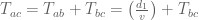
A method for two parties to verify if they share a common secret without revealing that secret if they don’t.

We didn’t cover zero knowledge proofs in the Security Engineering course I did last semester. But part way into the course I needed a way for two people, A and B to verify that some number they each know is infact the same number N in the case that they don’t have a trusted arbitrator and they don’t want to reveal the number they each know to the other person unless the other person has the same number.

I don’t think this is exactly a zero knowledge proof situation by it seems closely related. The motivating situation for this was a web application that set some cookies and I wanted to know if one of these cookies set was unique per user or unique per some other setting (but the web application doesn’t allow just anyone to create a new account, so I couldn’t determine this on my own). In the case that it was unique per user then I don’t want to tell anyone what my value for this cookie is because then they may be able to hijack my session.

So a method I thought of was that each person reveals one bit of the number to the other person at a time.

I’ll try to formalise this a bit more.

I’ll call this number the message. is the message knows, is the message knows. and arrange that they each know some message and arrange that they wish to verify if . If then and must each know that that is the case and if then and must also know (after conducting the verification) that this is the case, but do not wish to let the other one know what their message was.

and meet letting be the entity that begins the verification. Each message is first encoded into a binary representation using an agreed upon method. then tells what the 1st bit of is (denoted ). now verifies this bit with . If , tells the second bit of . If , randomly selects a bit (ie. randomly selects either 0 or 1) and tells that random bit instead, and flags that . As soon as either or flags that they subsequently always report a random bit regardless of whether the last bit reported to them was correct or not.

We could use an end of message token to indicate the end of the message. Of course this method isn’t perfect because if one’s random stream of bits matches what the other expects then one thinks that but the other thinks that .

Another problem is if both parties have determined that then when do they stop sending random bits to each other? If both parties are happy to reveal the length of their message then there is no problem. Otherwise both parties can keep sending random bits until they feel that the the message space they have opened up is large enough and they don’t mind revealing that the length of their message is less than the bit number they are up too.

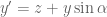
Here’s an example. A’s number is 0110. B’s number is 0110 and they want to check if they share the same number.

A -> B: 0 (B expects this)
B -> A: 1 (A expects this)
A -> B: 1 (B expects this)
B -> A: 0 (A expects this)
A -> B: $ (B expects this) (not needed if they first agree on revealing the message length)

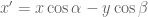
Another case A knows 0110, B knows 0010.

A -> B: 0 (B expects this)
B -> A: 0 (A does not expect this, so A concludes A_M != B_M, and subsequently sends randomness)
A -> B: Rand(0,1) (two cases)
    A sent 0 (B does not expect this, so B also concludes A_M != B_M, and subsequently sends randomness)
        ... continues until the end of M or until one party stops sending randomness.
    A sent 1 (B expects this, but A hasn't revealed anything as they made a random selection)
        B -> A: 0 (A doesn't know if B is sending randomness or not)
        if they agreed upon a message length,
            (A knows that A_M != B_M, but B thinks that A_M == B_M)
            (but A has only revealed 1 bit of A_M to B (because B doesn't know if A was sending A_M or randomness after the 1st bit),
             and B hasn't revealed anything of B_M to A (because A doesn't know if B was sending randomness))#
            (the probability of this happening is z)
        or, no message length agreed upon,
            A keeps sending randomness and B will detect this (because B is expecting the end of stream token and didn't get it), so they both know that A_M != B_M.

This is not very formal and I’m confident I’ve missed some details or left some a bit fuzzy, I only really wanted to explain the general concept.

# To be honest I’m not so sure if this is correct. Rather than me going around in circles unable to solve the math, and just abandoning this post, I’ll just leave it be and post with this uncertainty.

A Maths Problem: Transformed Horizontal Lines

This is the kind of post that I originally envisioned that I would post about when I started this blog. But after trying to complete this post I realised why I don’t do this very much, because I can’t always solve the problems I come up with. Anyway…

You can generate a funky kind of grid by taking a Cartesian coordinate system, joining lines from to for some values t. Here are some examples,

If you draw lots of lines you get something like,

Generated using code at http://github.com/andrewharvey/cairomisc/blob/bd41c8feb1beba38849878aed566c6f45a70856b/curved_grid_simple.pl

This is also what you get if you take a bunch of horizontal lines from to (where the horizontal lines are equally spaced above each other), and take all the endpoints from the line and rotate them about the point .

The thing I was interested in was as you draw more and more of these lines it looks like a curve emerges on the boundary. I imagined that if you drew infinitely many lines like these you would get a nice smooth curve. I want to know what is the formula for that curve. But as I started to try to work it out, it didn’t seem so simple.

I tried a lot of approaches, none of which seemed to work. So after a few initial set backs I tried to take a parametric approach taking t to be a value between 0 and 1 where this t indicates the line with start point . The point on the curve for this t is some point on that line. I tried to get that point via the intersection with the next line, ie. the point on this line that is also on the curve is between the intersection of that line and the line for and for some really small . But when I tried this approach as you make zero, then we get infinitely many points of intersection.

That didn’t work so easy but then I realised that if the point is on this line then (although I have not proved this but it seems obvious from the picture) that I have the gradient.

So all those lines as shown above have equation . (Except for t = 1 where we’ll just use a y value of 1). We can use this same t to define a point on the curve (which I call from here on) parametrically. So I assumed that the gradient of is given as . But now I’m not so sure that I have enough rigour here.

But then I got stuck again. I can try to go some integrals but this won’t work because you don’t know the relation between increasing t and the length along the curved you have moved. As you could have two different parametric functions which both have the same derivative function (ignoring the +c constant that disappears when you differentiate), just knowing the function defining the derivative of parametrically won’t tell me the equation of the original curve.

Moving on I now tried to calculate the area under the curve. I could partition it like how a Riemann integral is done.

We can easily calculate the area of any of these trapezoids (bounded by red). . We can get the x values by finding the point of intersection of the 2 lines that intersect at that x (and have the largest y value if there are several points of intersection for that x). Each line for some value t will have a point of intersection of the line before and after it (based on the t value). When I say the area of t = some number, I mean the area of the trapezoid starting with the intersection of the previous t line and ending with the intersection of the next t line. So the area of t = 1 is zero (because x₀ and x₁ are the same). The diagram above has . So,

Point A is the intersection of and , which is,

Point B is the intersection of and , which is,

So the area of this trapezoid is , which is

But then I got stuck here. I can compute a value for the approximate area.

phi = 0.0001;
area = 0;
for (t = 1; t > 0; t -= phi) {
   area += 2*t*t*phi*(1-t);
}
print area;

Which gives a value very close to 1/6, and if I integrate that area equation for t = 0..1 you get . But I don’t want the area, I want the formula that defines the area from x = 0 to some value x so that I can then differentiate this to get the equation of the original curve. So this is where I give up, and leave this for another day. If you work it out please post in the comments!

Oh and there is some rough code I wrote to make those images here. And a nice animation too.

MATH1081 and MATH1231 Cheat Sheets

Just cross posting my cheat sheets from MATH1081 and MATH1231. PDF and LaTeX source (WordPress.com won’t allow .tex uploads) are provided. These are from 08s2, at UNSW. I’ve released them into the public domain, if that is not legally possibly in Australia then lobby your parliament representative.

math1081.pdf

math1231-alg.pdf

math1231-calc.pdf

MATH1081 LaTeX Source

%This work is hereby released into the Public Domain. To view a copy of the public domain dedication, visit http://creativecommons.org/licenses/publicdomain/ or send a letter to Creative Commons, 171 Second Street, Suite 300, San Francisco, California, 94105, USA.

\documentclass[a4paper,10pt]{article}
\usepackage{verbatim}
\usepackage{amsmath}
\usepackage{amssymb}
\setlength\parindent{0mm}
\usepackage{fullpage}
\usepackage{array}
\usepackage[all]{xy}

\usepackage[pdftex,
            pdfauthor={Andrew Harvey},
            pdftitle={MATH1081 Cheat sheet 2008},
            pdfsubject={},
            pdfkeywords={}]{hyperref}

\begin{document}

\section*{Enumeration}
\subsection*{Counting Methods}
Let $\#(n)$ denote the number of ways of doing $n$ things. Then,
$$\#(A\; \mbox{and}\; B) = \#(A) \times \#(B)$$
$$\#(A\; \mbox{or}\; B) = \#(A) + \#(B)$$

($n$ items, $r$ choices)\\
Ordered selection with repetition, $n^r$.\\

Ordered selection without repetition, $P(n,r) = \frac{n!}{(n-r)!}$.\\

Unordered selection without repetition, $C(n,r) = \frac{P(n,r)}{r!}$.\\

$|A \cup B| = |A| + |B| - |A \cap B|$\\

Ordered selection with repeition; WOOLLOOMOOLOO problem.\\

Unordered selection with repetition; dots and lines,
$$\binom{n+r-1}{n-1}$$

Pigeonhole principle. If you have n holes and more than n objects, then there must be at least 1 hole with more than 1 object.

\section*{Recurrences}
\subsection*{Formal Languages}
$\lambda$ represents the \textit{empty word}.
$w$ is just a variable (it is not part of the language)

\subsection*{First Order Homogeneous Case}
The recurrence,\\
\begin{center}$a_n = ra_{n-1}$ with $a_0=A$\\\end{center}
has solution\\
$$a_n=Ar^n.$$

\subsection*{Second Order Recurrences}
$$a_n + pa_{n-1} + qa_{n-2} = 0$$
has characteristic,
$$r^2 + pr + q = 0$$
If $\alpha$ and $\beta$ are the solutions to the characteristic equation, and if they are real and $\alpha \ne \beta$ then,
$$a_n = A\alpha^n + B\beta^n.$$
If $\alpha = \beta$ then,
$$a_n = A\alpha^n + Bn\beta^n.$$

\subsection*{Guesses for a particular solution}
\begin{tabular}{c|c}%{m{width} | m{width}}
 LHS & Guess \\ \hline
$3$ & c \\
$3n$ & $cn + d$\\
$3\times 2^n$ & $c2^n$\\
$3n2^2$ & $(cn+d)2^n$\\
$(-3)^n$ & $c(-3)^n$\\
\end{tabular}

\end{document}

MATH1231-ALG LaTeX Source

%This work is hereby released into the Public Domain. To view a copy of the public domain dedication, visit http://creativecommons.org/licenses/publicdomain/ or send a letter to Creative Commons, 171 Second Street, Suite 300, San Francisco, California, 94105, USA.

\documentclass[a4paper,10pt]{article}
\usepackage{verbatim}
\usepackage{amsmath}
\usepackage{amssymb}
\setlength\parindent{0mm}
\usepackage{fullpage}

\usepackage[pdftex,
            pdfauthor={Andrew Harvey},
            pdftitle={MATH1231 Algebra Cheat sheet 2008},
            pdfsubject={},
            pdfkeywords={},
            pdfstartview=FitB]{hyperref}

\begin{document}

\section*{Vector Spaces}
\subsection*{Vector Spaces}
Vector Space - 10 rules to satisfy, including \begin{small}\textit{(Where $V$ is a vector space.)}\end{small}
\begin{itemize}
\item Closure under addition. If $\mathbf{u}, \mathbf{v} \in V$ then $\mathbf{u} + \mathbf{v} \in V$
\item Existence of zero. $\mathbf{0} \in V$
\item Closure under scalar multiplication. If $\mathbf{u} \in V$ then $\lambda \mathbf{u} \in V$, where $\lambda \in \mathbb{R}$
\end{itemize}

\subsection*{Subspaces}
Subspace Theorem:\\
  A subset $S$ of a vectorspace $V$ is a subspace if:
\begin{enumerate}
\renewcommand{\labelenumi}{\roman{enumi})}
\item $S$ contains the zero vector.
\item If $\mathbf{u}, \mathbf{v} \in S$ then $\mathbf{u} + \mathbf{v} \in S$ and $\lambda \mathbf{u} \in S$ for all scalars $\lambda$.
\end{enumerate}

\subsection*{Column Space}
The column space of a matrix $A$ is defined as the span of the columns of $A$, written $\mbox{col}(A)$.

\subsection*{Linear Independence}
Let $S = \{\mathbf{v_1}, \mathbf{v_2}, \dots, \mathbf{v_n}\}$ be a set of vectors.
\begin{enumerate}
\renewcommand{\labelenumi}{\roman{enumi})}
\item If we can find scalars $\alpha_1 + \alpha_2 + \dots + \alpha_n$ not all zero such that
\begin{center}$\alpha_1\mathbf{v_1} + \alpha_2\mathbf{v_2} + \dots + \alpha_n\mathbf{v_n} = 0$\end{center}
then we call $S$ a linearly dependent set and that the vectors in $S$ are linearly dependent.

\item If the only solution of
\begin{center}$\alpha_1\mathbf{v_1} + \alpha_2\mathbf{v_2} + \dots + \alpha_n\mathbf{v_n} = 0$\end{center}
is $\alpha_1 = \alpha_2 = \dots = \alpha_n = 0$ then $S$ is called a linearly independent set and that the vectors in $S$ are linearly independent.
\end{enumerate}

\subsection*{Basis}
A set $B$ of vectors in a vectorspace $V$ is called a basis if
\begin{enumerate}
\renewcommand{\labelenumi}{\roman{enumi})}
\item $B$ is linearly independent, and
\item $V = \mbox{span}(B)$.
\end{enumerate}

An orthonormal basis is formed where all the basis vectors are unit length and are mutually orthogonal (the dot product of any two is zero).

\subsection*{Dimension}
The dimension of a vectorspace $V$, written dim($V$) is the number of basis vectors.

\section*{Linear Transformations}
\subsection*{Linear Map}
A function $T$ which maps from a vectorspace $V$ to a vectorspace $W$ is said to be linear if, for all vectors $\mathbf{u}, \mathbf{v} \in V$ and for any scalar $\lambda$,
\begin{enumerate}
\renewcommand{\labelenumi}{\roman{enumi})}
\item $T(\mathbf{u} + \mathbf{v}) = T(\mathbf{u}) + T(\mathbf{v})$,
\item $T(\lambda\mathbf{u}) = \lambda T(\mathbf{u})$.
\end{enumerate}

The columns of the transformation matrix are simply the images of the standard basis vectors.

\subsection*{The Kernel}
$\mbox{im}(T) = \mbox{col}(A)$\\
The kernel of a linear map $T : V \to W$, written ker($T$), consists of the set of vectors $\mathbf{v} \in V$ such that $T(\mathbf{v}) = \mathbf{0}$.\\
If A is the matrix representation of a linear map $T$, then the kernel of $A$ is the solution set of $A\mathbf{x} = \mathbf{0}$.

\subsection*{Rank-Nullity}
The dimension of the image of a linear map $T$ is called the rank of $T$, written rank($T$). (Maximum number of linearly independent columns of A)\\

The dimension of the kernel of a linear map $T$ is called the nullity of $T$, written nullity($T$). (Number of parameters in the solution set of $A\mathbf{x}=\mathbf{0}$)\\

If $T$ is a linear map from $V$ to $W$ then
$$\mbox{rank}(T) + \mbox{nullity}(T) = \mbox{dim}(V)$$

\section*{Eigenvectors and Eigenvalues}
If $A$ is a square matrix, $\mathbf{v} \ne 0$ and $\lambda$ is a scalar such that,
$$A\mathbf{v} = \lambda\mathbf{v}$$
then $\mathbf{v}$ is an eigenvector of $A$ with eigenvalue $\lambda$.\\
\begin{comment}
\begin{equation*}
A\mathbf{v} = \lambda\mathbf{v}
\implies (A-\lambda I)\mathbf{v} = \mathbf{0}

A-\lambda I \mbox{has no inverse (otherwise } \mathbf{v} = \mathbf{0} \mbox{)}
\mbox{so set det}(A-\lambda I) = 0
 \mbox{this finds the eigenvectors}

\mbox{Also since}
(A-\lambda I)\mathbf{v} = \mathbf{0}
\mathbf{v} \in \mbox{ker}(A-\lambda I)
\mbox{this gives eigenvectors.}
\end{equation*}
\end{comment}
Eigenvalues: Set $\mbox{det}(A-\lambda I) = 0$ and solve for $\lambda.$\\
Eigenvectors: For each value of $\lambda$ find the kernel of $(A-\lambda I)$.

\subsection*{Diagonalisation}
If $A$ has $n$ (independent) eigenvectors then put,\\
$P = (\mathbf{v_1}|\mathbf{v_2}|...|\mathbf{v_n})$ (eigenvectors $\mathbf{v}$)\\
and\\
$D =
\begin{pmatrix}
  \lambda_1 &        & 0         \\
            & \ddots &           \\
  0         &        & \lambda_n
\end{pmatrix}
$ (eigenvalues $\lambda$)\\
\\
so then\\
$A^k = PD^kP^{-1}$, for each non-negative integer $k$.\\
\\
Remember that when $A =
\bigl( \begin{smallmatrix}
  a&b\\ c&d
\end{smallmatrix} \bigr)$, $A^{-1} = \frac{1}{det(A)}
\begin{pmatrix}
d & -b\\
-c & a\end{pmatrix}$

\subsection*{Systems of Differential Equations}
The system
$\begin{cases}
	\frac{dx}{dt} = 4x + y\\
	\frac{dy}{dt} = x + 4y
\end{cases}$
 can be written $\mathbf{x}'(t) = \begin{pmatrix} 4 & 1\\1 & 4\end{pmatrix}\mathbf{x}(t)$ where $\mathbf{x}(t) = \binom{x(t)}{y(t)}.$

We can guess the solution to be $\mathbf{x}(t) = \alpha \mathbf{v} e^{\lambda t}$ (and add for all the eigenvalues). Where $\mathbf{v} $ and $ \lambda$ are the eigenvectors and eigenvalues respectively.

\section*{Probability and Statistics}

\subsection*{Probability}
Two events $A$ and $B$ are mutually exclusive if $A \cap B = \emptyset$.
$$P(A^c) = 1 - P(A)$$
$$P(A \cup B) = P(A) + P(B) - P(A \cap B)$$

\subsection*{Independence}
Two events $A$ and $B$ are physically independent of each other if the probability that one of them occurs is not influenced by the occurrence or non occurrence of the other. These two events are statistically independent if, $$P(A \cap B) = P(A).P(B).$$

\subsection*{Conditional Probability}
Probability of $A$ given $B$ is given by,
$$P(A|B) = \frac{P(A \cap B)}{P(B)}$$

\subsection*{Bayes Rule}

\subsection*{Discrete Random Variables}
$$p_k = P(X=k) \qquad \mbox{(} \{p_k\}\mbox{ is the probability distribution)}$$
where, $X$ is a discrete random variable, and $P(X=k)$ is the probability that $X=k$.\\

For $\{p_k\}$ to be a probability distribution,
\begin{enumerate}
\renewcommand{\labelenumi}{\roman{enumi})}
\item $p_k \ge 0$ for $k = 0, 1, 2, \dots$
\item $p_0 + p_1 + \dots = 1$
\end{enumerate}

\subsection*{Mean and Variance}
$E(X)$ denotes the mean or expected value of X.\\
%$$E(X) = \sum_{i=1}^{k} p_i x_i \qquad  $$
$$E(X) = \sum_{\mbox{all }k} kp_k$$

$$\mbox{Var}(X) = E(X^2) - E(X)^2 \qquad \mbox{where } E(X^2) = \sum_{\mbox{all } k} k^2 p_k$$

\subsection*{Binomial Distribution}
If we perform a binomial experiment (i.e. 2 outcomes) $n$ times, and each time there is a probability $p$ of success then,
$$P(X=k) = \binom{n}{k} p^k (1-p)^{n-k},\qquad \mbox{for } 0\le k \le n \mbox{ and 0 otherwise}.$$

\subsection*{Geometric Distribution}
$$P(X=k) = p(1-p)^{k-1}, \;\; k = 1, 2, \dots$$
\end{document}

MATH1231-CACL LaTeX Source

%This work is hereby released into the Public Domain. To view a copy of the public domain dedication, visit http://creativecommons.org/licenses/publicdomain/ or send a letter to Creative Commons, 171 Second Street, Suite 300, San Francisco, California, 94105, USA.

\documentclass[a4paper,10pt]{article}
\usepackage{verbatim}
\usepackage{amsmath}
\usepackage{amssymb}
\setlength\parindent{0mm}
\usepackage{fullpage}
\usepackage[all]{xy}

\usepackage[pdftex,
pdfauthor={Andrew Harvey},
pdftitle={MATH1231 Calculus Cheat sheet 2008},
pdfsubject={},
pdfkeywords={},
pdfstartview=FitB]{hyperref}

\begin{document}
\section*{Functions of Several Variables}
\subsection*{Sketching}
\begin{itemize}
\item Level Curves
\item Sections
\end{itemize}

\subsection*{Partial Derivatives}
$$\frac{\partial^2 f}{\partial y \partial x} = \frac{\partial^2 f}{\partial x \partial y}$$
on every open set on which $f$ and the partials,\\
$$\frac{\partial f}{x}, \frac{\partial f}{y}, \frac{\partial^2 f}{\partial y \partial x}, \frac{\partial^2 f}{\partial x \partial y}$$
are continuous.

\subsection*{Normal Vector}
$$\mathbf{n} = \pm
\begin{pmatrix}
\frac{\partial f(x_0, y_0)}{\partial x}\\
\frac{\partial f(x_0, y_0)}{\partial y}\\
-1\\
\end{pmatrix}
$$

\subsection*{Error Estimation}
$$f(x_0 + \Delta x, y_0 + \Delta y) \approx f(x_0, y_0) + \left[ \frac{\partial f}{\partial x} (x_0, y_0)\right] \Delta x + \left[ \frac{\partial f}{\partial y} (x_0, y_0)\right] \Delta y$$

\subsection*{Chain Rules}
Example, $z = f(x,y)\ \mbox{with}\ x = x(t), y = y(t)$
\begin{displaymath}
\xymatrix{
& f \ar[dl] \ar[dr] &   \\
x \ar[d] &                   & y \ar[d]\\
t        &                   & t}
\end{displaymath}

$$\frac{df}{dt} = \frac{\partial f}{\partial x} \cdot \frac{dx}{dt} + \frac{\partial f}{\partial y} \cdot \frac{dy}{dt}$$

\section*{Integration}
\subsection*{Integration by Parts}
Integrate the chain rule,
$$u(x)v(x) = \int u'(x)v(x)\; dx + \int v'(x)u(x)\; dx$$

\subsection*{Integration of Trig Functions}
For $\int \sin^2 x\; dx$ and $\int \cos^2 x\; dx$ remember that,\\
$$\cos 2x = \cos^2 x - \sin^2 x$$
%$$\sin 2x = 2\sin x \cos x$$

Integrals of the form $\int \cos^m x \sin^n x\; dx$, when $m$ or $n$ are odd, you can factorise using $\cos^2 x + \sin^x = 1$  and then using,
$$\int \sin^k x \cos x\; dx = \frac{1}{k+1} \sin^{k+1} x + C$$
$$\int \cos^k x \sin x\; dx = \frac{-1}{k+1} \cos^{k+1} x + C$$

\subsection*{Reduction Formulae}
...

\subsection*{Partial Fractions}
Example, assume
$$\frac{2x-1}{(x+3)(x+2)^2} = \frac{A}{x+3} + \frac{Bx + C}{(x+2)^2}$$
\begin{comment}
\begin{enumerate}
\renewcommand{\labelenumi}{\roman{enumi})}
\item $\frac{2x-1}{x+2} = A + \frac{B(x+3)}{x+2}$ subs $x=-3 \to A=7$
\item $\frac{2x-1}{x+3} = \frac{A(x+2)}{x+3} + B$ subs $x=-2 \to B=-5$
\end{enumerate}
\end{comment}
Now multiply both sides by $(x+2)(x+3)$ and equate coefficients.

\section*{ODE's}
\subsection*{Separable ODE}
Separate then integrate.

\subsection*{Linear ODE}
The ODE:
$$ \frac{dy}{dx} + f(x)y=g(x) $$
has solution,
$$ y(x) = \frac{1}{u(x)}\left [ \int u(x)g(x)\ dx + C \right] $$
where,
$$ u(x) := e^{\int f(x)\ dx} $$

\subsection*{Exact ODE}
The ODE:
$$ \frac{dy}{dx} = -\frac{M(x,y)}{N(x,y)} $$
or as,
$$ M(x,y)dx + N(x,y)dy = 0 $$
is exact when,
$$ \frac{\partial M}{\partial y} = \frac{\partial N}{\partial x} $$

Assume solution is of the form,
$$ F(x,y) = c $$
with,
$$ M = \frac{\partial F}{\partial x} \qquad N = \frac{\partial F}{\partial y}$$

Integrate to find two equations equal to $F(x,y)$, then compare and find solution from assumed form.

\subsection*{Second Order ODE's}
The ODE:
$$ay'' + ay' + by = f(x)$$
For the homogeneous case ($f(x) = 0$)\\
the characteristic equation will be $a\lambda^2 + b\lambda + c = 0$

If the characteristic equation has,\\
Two Distinct Real roots, (replace the $\lambda$'s with the solutions to the characteristic eqn.)
$$ y = Ae^{\lambda x} + Be^{\lambda x}$$

Repeated Real roots,
$$ y = Ae^{\lambda x} + Bxe^{\lambda x}$$

Complex roots,
$$ y = e^{\alpha x}(A\cos \beta x + B\sin \beta x)$$

where,
$$\lambda = \alpha \pm \beta i$$

For the For the homogeneous case,
$$y = y_h + y_p$$
$$y = \mbox{solution to homogeneous case} + \mbox{particular solution}$$

Guess something that is in the same form as the RHS.\\
If $f(x) = P(x)\cos ax \mbox{(or sin)}$ a guess for $y_p$ is $Q_1(x)\cos ax + Q_2(x)\sin ax$

\section*{Taylor Series}
\subsection*{Taylor Polynomials}
For a differentiable function $f$ the Taylor polynomial of order $n$ at $x=a$ is,
$$P_n(x) = f(a) + f'(a)(x-a) + \frac{f''(a)}{2!}(x-a)^2 + \dots + \frac{f^{\left( n\right) }(a)}{n!}(x-a)^n$$

\subsection*{Taylor's Theorem}
$$f(x) = f(a) + f'(a)(x-a) + \frac{f''(a)}{2!}(x-a)^2 + \dots + \frac{f^{\left( n\right) }(a)}{n!}(x-a)^n + R_n(x)$$

where,\\
$$R_n(x) = \frac{f^{\left( n+1\right) }(c)}{(n+1)!}(x-a)^{n+1}$$

\subsection*{Sequences}
$$\lim_{x \to \infty} f(x) = L \implies \lim_{n \to \infty}a_n = L$$
essentially says that when evaluating limits functions and sequences are identical.

A sequence diverges when $\displaystyle \lim_{n \to \infty}a_n = \pm \infty$ or $\displaystyle \lim_{n \to \infty}a_n$ does not exist.

\subsection*{Infinite Series}
\subsubsection*{Telscoping Series}
Most of the terms cancel out.

\subsubsection*{$n$-th term test (shows divergence)}
$\displaystyle \sum_{n=1}^{\infty} a_n$ diverges if $\displaystyle \lim_{n \to \infty}{a_n}$ fails to exist or is non-zero.

\subsubsection*{Integral Test}
Draw a picture. Use when you can easily find the integral.

\subsubsection*{$p$- series}
The infinite series $\displaystyle \sum_{n=1}^{\infty} \frac{1}{n^p}$ converges if $p>1$ and diverges otherwise.

\subsubsection*{Comparison Test}
Compare to a p-series.

\subsubsection*{Limit form of Comparison Test}
Look at $\displaystyle \lim_{n \to \infty}{\frac{a_n}{b_n}}\;$ where $b_n$ is usually a p-series.\\
If $=c>0$, then $\sum a_n$ and $\sum b_n$ both converge or both diverge.\\
If $=0$ and $\sum b_n$ converges, then $\sum a_n$ converges.\\
If $=\infty$ and $\sum b_n$ diverges, then $\sum a_n$ diverges.

\subsubsection*{Ratio Test}
$$\lim_{n \to \infty} \frac{a_{n+1}}{a_n} = \rho$$

The series converges if $\rho < 1$,\\
the series diverges if $\rho > 1$ or $\rho$ is infinite,\\
and the test is inconclusive if $\rho = 1$.

\subsubsection*{Alternating Series Test}
The series,
$$\sum_{n=1}^{\infty} (-1)^{n+1} u_n = u_1 - u_2 + u_3 - u_4 + \dots$$
converges if,
\begin{enumerate}
\item The $u_n$'s are all $>0$,
\item $u_n \ge u_{n+1}$ for all $n \ge N$ for some integer $N$, and
\item $u_n \rightarrow 0$.
\end{enumerate}

\subsubsection*{Absolute Convergence}
If $\displaystyle \sum_{n=1}^{\infty} |a_n|$ converges, then $\displaystyle \sum_{n=1}^{\infty} a_n$ converges.

\subsection*{Taylor Series}
Taylor Polynomials consist of adding a finite number of things together, whereas Taylor Series is an infinite sum.\\
The Maclaurin series is the Taylor series at $x=0$.
\subsection*{Power Series}

\section*{More Calculus}
\subsection*{Average Value of a Function}
$$\frac{\displaystyle \int_a^b f(x)\ dx}{b-a}$$

\subsection*{Arc Length}
\begin{center}
Arc length over $\displaystyle[a,b] = \int_a^b \sqrt{1+f'(x)^2}\ dx$\\
\end{center}
$$s = \int_a^b \sqrt{x'(t)^2 + y'(t)^2}\ dt \qquad \mbox{(parametric)}$$

\subsection*{Speed}
$$\frac{ds}{dt} = \sqrt{x'(t)^2 + y'(t)^2}$$

\subsection*{Surface Area of Revolution}
$$2\pi \int_a^b f(x) \sqrt{1+f'(x)^2}\ dx$$
$$2\pi \int_a^b y(t) \sqrt{x'(t)^2 + y'(t)^2}\ dt \qquad \mbox{(parametric)}$$
\end{document}

A Response to Terence Tao’s “An airport-inspired puzzle”

In Terence Tao’s latest post he poses three questions. Here are my solutions.

Suppose you are trying to get from one end A of a terminal to the other end B.  (For simplicity, assume the terminal is a one-dimensional line segment.)  Some portions of the terminal have moving walkways (in both directions); other portions do not.  Your walking speed is a constant v, but while on a walkway, it is boosted by the speed u of the walkway for a net speed of v+u.  (Obviously, one would only take those walkway that are going in the direction one wishes to travel in.)  Your objective is to get from A to B in the shortest time possible.

1. Suppose you need to pause for some period of time, say to tie your shoe.  Is it more efficient to do so while on a walkway, or off the walkway?  Assume the period of time required is the same in both cases.
2. Suppose you have a limited amount of energy available to run and increase your speed to a higher quantity v’ (or v’+u, if you are on a walkway).  Is it more efficient to run while on a walkway, or off the walkway?  Assume that the energy expenditure is the same in both cases.
3. Do the answers to the above questions change if one takes into account the effects of special relativity?  (This is of course an academic question rather than a practical one.)

Source: Terence Tao, http://terrytao.wordpress.com/2008/12/09/an-airport-inspired-puzzle/

Q1.

After just thinking about it without any mathematics I was not to sure so I used a mathematical approach. The first thing I did was to draw a diagram,

Admittedly, I did simplify the problem in my diagram, however I am confident that this will not affect the final answer. (How do I prove this? I don’t know.) Along with this diagram I also had to define some things in terms of variables.

As shown in the diagram, A is the starting point, B is the ending point, C is an arbitrary point in between which separates the escalator section from the non-escalator sections.

Let,
t = time it takes to tie shoe lace
v = walking speed
u = escalator speed
= time it takes to get from A to C
= time it takes to get from C to B
= time it takes to get from A to B

We also know, .

Now lets consider two scenarios. Scenario A, the person ties their shoe lace in the non-escalator section. Scenario B, the person ties their shoe lace in the escalator section.

Scenario A:

Scenario B:

Now let

I shall now make some reasonable assumptions (also formalising things a bit more),

All variables are real, and we shall assume that the person has time to tie their shoe lace while on the escalator. I.e.

I shall denote to be from scenario A and to be from scenario B. Now to see which is larger or we can examine the sign of . If it is positive then , if it is negative then .

By some algebra and as ,  . Hence . Therefore it would be more efficient pause for a moment while on an escalator walkway.\

Q2.

I will take a similar approach for Q2, examining the two cases and then comparing the resultant time.

(I’ll re-edit the post when I get around to working out the solution)

The Mathematics Behind Graphical Drawing Projections in Technical Drawing

In the field of technical drawing, projection methods such as isometric, orthogonal, perspective are used to project three dimensional objects onto a two dimensional plane so that three dimensional objects can be viewed on paper or a computer screen. In this article I examine the different methods of projection and their mathematical roots (in an applied sense).

The approach that seems to be used by Technical Drawing syllabuses in NSW to draw simple 3D objects in 2D is almost entirely graphical. I don’t think you can say this is a bad thing because you don’t always want or need to know the mathematics behind the process, you just want to be able to draw without thinking about this. However to have an appreciation of what’s really happening the mathematical understanding is a great thing to learn.

Many 3D CAD/CAM packages available on the market today (such as AutoCAD, Inventor, Solidworks, CATIA, Rhinoceros) can generate isometric, three point perspective or orthogonal drawings from 3D geometry, however from what I’ve seen they can’t seem do other projections such as dimetric, trimetric, oblique, planometric, one and two point perspective. Admittedly I don’t think these projections are any use or even needed, but when your at high school and you have to show that you know how do to oblique, et al. it can be a problem when the software cannot do it for you from your 3D model. (So I actually wrote a small piece of software to help with this in this article). But to do so, I needed to understand the mathematics behind these graphical projections. So I will try to explain that here.

The key idea is to think of everything having coordinates in a coordinate system (I will use the Cartesian system for simplicity). We can then express all these projections as mathematical transformations or maps. Like a function, you feed in the 3D point, and then you get out the projected 2D point. Things get a bit arbitrary here because an isometric view is essentially exactly the same as a front view. So we keep to the convention that when we assign the axis of the coordinate system we try to keep the three planes of the axis parallel to the three main planes of the object.

The three "main" planes of the object are placed parallel to the three planes of the axis. This is how we will choose our axis in relation to the object.

We will not do this though,

We will not choose it like this...

...or this.

In fact doing something like that shown just above with the object rotated is how we get projections like isometric.

Now what we do is take the coordinates of each point and “transform” them to get the projected coordinates, and join these points with lines where they originally were. However we can only do this for some kinds of projections, indeed for all the ones I have mentioned in this post this will do but only because these projections have a special property. They are linear maps (affine maps also hold this property and are a superset of the set of linear maps) which means that straight lines in 3D project to straight lines in 2D.

For curves we can just project a lot of points on the curve (subdivide it) and then join them up after they are projected. It all depends what our purpose is and if we are applying it practically. We can generate equations of the projected curves if we know the equation of the original curve but it won’t always be as simple. For example circles in 3D under isometric projection become ellipses on the projection plane.

Going back to the process of the projection, we can use matrices to represent these projections where

is the same as,

We call the 3 by 3 matrix above as the matrix of the projection.

Knowing all this, we can easily define orthogonal projection as you just take two of the dimensions and cull the third. So for say an orthographic top view the projection matrix is simply,

Now we want a projection matrix for isometric. One way would be to do the appropriate rotations on the object then do an orthographic projection, we can get the projection matrix by multiplying the matrices for the rotations and orthographic projection together. However I will not detail that here. Instead I will show you another method that I used to describe most of the projections that I learnt from high school (almost all except perspectives).

I can describe them as well as many “custom” projections in terms of what the three projected axis look like on the projection plane. I described them all in terms of a scale on each of the three axis, as well as the angle two of the axis make with the projection plane’s horizontal.

Projection attributes described in terms of the projected axis.

Using this approach we can think of the problem back in a graphical perspective of what the final projected drawing will look like rather than looking at the mathematics of how the object gets rotated prior to taking an orthographic projection or what angle do the projection lines need to be at in relation to the projection plane to get oblique, etc. Note also that the x, y, z in the above diagram are the scales of the x, y, z axis respectively. So we can see in the table below that we can now describe these projections in terms of a graphical approach that I was first taught.

Projection	α (alpha)	β (beta)	Sx	Sy	Sz
Isometric	30°	30°	1	1	1
Cabinet Oblique	45°	0°	0.5	1	1
Cavalier Oblique	45°	0°	1	1	1
Planometric	45°	45°	1	1	1

Now all we need is a projection matrix that takes in alpha, beta and the three axes scale’s and does the correct transformation to give the projection. The matrix is,

Now for the derivation. First we pick a 3D Cartesian coordinate system to work with. I choose the Z-up Left Hand Coordinate System, shown below and we imagine a rectangular prism in the 3D coordinate system.

Block in 3D coordinate system.

Now we imagine what it would look like in a 2D coordinate system using isometric projection.

Block in 2D coordinate system (isometric).

As the alpha and beta angles (shown below) can change, and therefore not limited to a specific projection, we need to use alpha and beta in the derivation.

Now using these simple trig equations below we can deduce the following.

All the points on the xz plane have y = 0. Therefore the x’ and y’ values on the 2D plane will follow the trig property shown above, so:

However not all the points lie on the xz plane, y is not always equal to zero. By visualising a point with a fixed x and z value but growing larger in y value, its x’ will become lower, and y’ will become larger. The extent of the x’ and y’ growth can again be expressed with the trig property shown, and this value can be added in the respective sense to obtain the final combined x’ and y’ (separately).

If y is in the negative direction then the sign will automatically change accordingly. The next step is to incorporate the scaling of the axes. This was done by replacing the x, y & z with a the scale factor as a multiple of the x, y & z. Hence,

This can now easily be transferred into matrix form as shown at the start of this derivation or left as is.

References:
Harvey, A. (2007). Industrial Technology – Graphics Industries 2007 HSC Major Project Management Folio. (Link)

An Introduction to Hypercubes.

Point, Line Segment, Square, Cube. But what comes next, what is the equivalent object in higher dimensions? Well it is called a hypercube or n-cube, although the 4-cube has the special name tesseract.

Construction Methods

Before I go on to explain about the elements of hypercubes, let me show you some pictures of some hypercubes. I guess this also raises the question how can you construct these objects. One method is to start with a point. Then stretch it out in one dimension to get a line segment. Then take this line and stretch it out in another dimension perpendicular to the previous one, to get a square. Then take that square and stretch it out in another dimension perpendicular to the previous two to get a cube. This is when your visualisation may hit a wall. Its very hard to then visualise taking this cube and stretching it in another dimension perpendicular to the previous three. However mathematically, this is easy and this is one approach to constructing hypercubes.

We place a point in R3.

...and then stretch the point in one dimension to make a line...

...and then we stretch that line in a direction perpendicular to the previous time...

...and finally stretch that plane in a direction perpendicular the the previous two times.

However there is more mathematical and analytical method. You most probably know that these n-cubes have certain elements to them, namely vertices (points), edges (lines), faces (planes), and then in the next dimension up, cells and then in general n-faces. These elements are summed up nicely here. Firstly we take a field of say . Next we construct the vertices of the n-cube. Basically we are taking all the n dimensional vectors which have all the combinations of 0’s and 1’s for each entry of the vector. More mathematically,
There is a vertex described by each vector where
There is an edge between vertices and if and only if for exactly one .

There is an m-face between (or though) vertices and and … and if and only if for exactly .

Basically this means we list the vertices just as if were were counting in base 2. And then we can group these vertices into different groups based on the n-face level and (if we think of the vertices of a bit string) how many bits we have to change to make two vertices bit streams the same. This approach is very interesting because the concept of grouping these vertices relates strongly to hypergraphs.

Another way to think about it is as follows. Edges, from the set of all edges (i.e. joining each vertex with every other vertex), are the ones that are perpendicular to one of the standard basis vectors. This generalises to n-faces; from the set of all n-faces (i.e. all ways of grouping vertices into groups of n) are those that the object constructed is parallel to the span of any set of n of the standard basis vectors.

When you think about it, a lot of things that you can say about the square or cube generalise. For instance you can think of a square being surrounded by 4 lines, and cube by 6 surfaces, a tesseract by 8 cells, etc.

Visualisation Methods

Now that we have some idea how to describe and build n-cubes, the next question is how do we draw them. There are numerous methods and I can’t explain them all in this post (such as slicing and stereographic projection, as well as other forms of projection (I’ll leave these for another blog article)). But another question is also what aspects do we draw and how do we highlight them. For instance it may seem trivial in two dimensions to ask do I place a dot at each vertex and use just 4 solid lines for the edges. But in higher dimensions we have to think about how do we show the different cells and n-faces.

Firstly, how can we draw or project these n dimensional objects in a lower dimensional world (ultimately we want to see them in 2D or 3D as this is the only space we can draw in). This first method is basically the exact same approach that most people would have first learnt back in primary school. Although, I do not think it makes the most sense or makes visualisation easiest. Basically this method is just the take a dot and perform a series of stretches on it that I described earlier, although most people wouldn’t think this is what they were doing. Nor would we usually start with a dot, we would normally start with the square. Although we will, so we start with this.

0-cube.

We would now draw a line along some axis from that dot, and place another dot at the end of this line.

1-cube, showing vertices and edges.

Now from each of the dots we have, we would draw another line along some other axis and again draw a dot at the end of each of those two lines. We would then connect the newly formed dots.

2-cube, showing vertices and edges.

Now, we just keep repeating this process where by each time we are drawing another dimension. So we take each of these four dots and draw lines from them in the direction of another axis, placing a dot at the end of each of these lines, and joining each of the dots that came from other dots that were adjacent, with a line.

3-cube, showing vertices and edges.

Now for 4D and beyond we basically keep the process going, just choosing really anywhere from the new axis, so long as it passes though the origin.

4-cube, showing vertices and edges.

If we do a little bit of work we can see that this map is given by the matrix,

where is the angle of the projected z axis from the x axis, and is the angle of the projected w axis from the negative x axis. Also r₁ and r₂ are the scales of the third and fourth respective receding axis (it makes it “look” more realistic when we use a number less than 1) This is just an extension of oblique projection for 3D to 2D.

Now this method seems very primitive, and a much better approach is to use all the dimensions we have. We live in a three dimensional world, so why just constrict our drawings to two dimensions! Basically, an alternate approach to draw an n-cube in three dimensional space would be to draw n lines all passing though a single point. Although it is not necessary to make all these lines as spread out as possible, we will try to. (This actually presents another interesting idea of how do we equally distribute n points on a sphere. For instance we can try to make it so that all the angles between any two of the points and the origin are equal. But I will leave this for another blog article later.) We then treat each of these lines as one dimension from there we can easily draw, or at least represent an n-dimensional point in 3D space. Now obviously we can have two different points in 4D that map to the same 3D point, but that is always going to happen no matter what map we use. The following set of 4 vectors are the projected axis we will use as a basis.

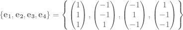
Now I won’t say how I got these (actually I took them from Wikipedia, they are just the vertices of a 3-simplex) but all of the vectors share a common angle between any two and the origin.

Now if we draw in our tesseract, highlighting the cells with different colours (not this became problematic with some faces and edges as they are a common boundary for two different faces, so you cannot really make them one colour or the other) we get something like this,

Tesseract projected onto R3. The cells are shown in different colours, the purple lines show the four axis.

The projection matrix for this projection is then simply (from the vectors that each of the standard basis maps to),

Now if we compare this to our original drawing (note I’m not talking about the projection used, but rather the presentation of the drawings, i.e. the colour.) I think you will see that the second one is clearer and try’s to show where the cells and faces are, not just the vertices and edges. Note also the second one is in 3D so you can rotate around it. Looking at the first one though, you will notice it doesn’t show where the faces or cells are. Remember that we have more than just vertices, edges and faces. We have cells, and n-faces. These are essentially just different groupings of the vertices. But how can we show these. Now the most mathematical way would be to just list all the different groupings. This is okay, but I like to see things in a visual sense. So another way would just show different elements. Like you draw all the vertices on one overhead, edges on another, and so on. Then when you put all these overheads on top of each other we get the full image, but we can also look at just one at a time to see things more clearly. This would be particularly more useful for the higher dimensional objects and higher dimensional elements. We can also use different colours to show the different elements. For example in the square, we can see that the line around surrounding it is 4 lines, but in higher dimensions its not so easy, so we can colour the different parts to the element differently. (When I say part I mean the 4 edges of a square are 4 different parts. Whereas the edges are all one element, but are a different element to the vertices.)

Some Interesting Properties

Once you start defining hypercubes there are many interesting properties that we can investigate. For this section lets just assume that we have the standard hypercube of side length 1. Now we can trivially see that the area, volume, etc. for the respective hypercube will always be 1. As described above each time we add another dimension and sweep the object out into that dimension we effectively multiply this hypervolume by 1. So for an n-cube, the hypervolume of it will be . When I say hypervolume I mean the one that makes sense for that dimension. E.g. in 2D, area, in 3D, volume, and so on.

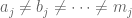
The next obvious question to ask is what is the perimeter, surface area, cell volume, …, n-face hypervolume of the respective n-cube? It gets a little confusing as you have to think about what exactly you are finding. Is it a length, an area, a volume? Well it will just be an (n – 1) volume. Eg. in 2D we are finding a length (the perimeter), in 3D, an area (surface area), and so on so that each time we increase the dimension of the n-cube we increase the units we are measuring in. Well if we just start listing the sequence (starting with a square), 4, 6… we notice this is just the number of (n – 1) degree elements. Namely, the number of edge, faces, cells, etc.

This leads me in the obvious question of how can I calculate the number of m-elements of the n-cube?

Well instead of me just going to the formula, which you can find on Wikipedia anyway, I will go though my lines of thinking when I first tried to work this out. Number of vertices is easy, each component of the n-vector can be either a 0 or a 1. So for each component there is 2 possibilities, but we have n of them, so it is just 2x2x2… n times, or 2ⁿ. Now originally when I tried to work out the number of edges, I started listing them and saw that I could construct the recurrence… Although with the help of graph theory it is very simple. In graph theory the handshaking theorem says 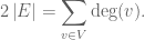Where means the number of edges, and means the degree of vertex V, which means the number of edges connected two it. Now if we think of an edge being a group of two vertices where you only make one entry of the vector change to get from one vector to the other, then we can see that there are exactly n way of doing this. We can either change the 1st entry of the vector, or the 2nd, or the …., or the nth. Thus each vertex has of the n-cube graph will have degree n. So as we have 2ⁿ vertices and each vertex has degree n, then the sum of the vertex degrees will be n2ⁿ. Hence by the handshaking theorem, I am not exactly sure how to generalise this further. I will leave it for another article. However, the formula is

(I shall try to write more at a later date.)

References:

• Hypercube. (2008, October 14). In Wikipedia, The Free Encyclopedia. Retrieved 08:19, October 21, 2008, from http://en.wikipedia.org/w/index.php?title=Hypercube&oldid=245242295
• Tran, T., & Britz, T. (2008). MATH1081 Discreet Matematics: 5 Graph Theory.